Distance to nearest neighbor
Estimating the optimal distance threshold for partitioning clonally related sequences is accomplished by calculating the distance from each sequence in the data set to its nearest neighbor and finding the break point in the resulting bi-modal distribution that separates clonally related from unrelated sequences. This is done via the following steps:
- Calculating of the nearest neighbor distances for each sequence.
- Generating a histogram of the nearest neighbor distances followed by either manual inspect for the threshold separating the two modes or automated threshold detection.
Example data
A small example AIRR Rearrangement database is included in the alakazam package.
Calculating the nearest neighbor distances requires the following
fields (columns) to be present in the table:
sequence_idv_callj_calljunctionjunction_length
# Subset example data to one sample
library(shazam)
data(ExampleDb, package="alakazam")
Calculating nearest neighbor distances (heavy chain sequences)
By default, distToNearest, the function for calculating distance between every
sequence and its nearest neighbor, assumes that it is running under non-single-cell
mode and that every input sequence is a heavy chain sequence and will be used for
calculation. It takes a few parameters to adjust how the distance is measured. If a
genotype has been inferred using the methods in the tigger package, and a
v_call_genotyped field has been added to the database, then this column may be
used instead of the default v_call column by specifying the vCallColumn
argument. This will allows the more accurate V call from tigger to be used for
grouping of the sequences. Furthermore, for more leniency toward ambiguous
V(D)J segment calls, the parameter first can be set to FALSE. Setting
first=FALSE will use the union of all possible genes to group sequences, rather
than the first gene in the field. The model parameter determines which
underlying SHM model is used to calculate the distance. The default model is
single nucleotide Hamming distance with gaps considered as a match to any
nucleotide (ham). Other options include a human Ig-specific single nucleotide
model similar to a transition/transversion model (hh_s1f) and the corresponding
5-mer context model from Yaari et al, 2013 (hh_s5f), an analogous pair of
mouse specific models from Cui et al, 2016 (mk_rs1nf and mk_rs5nf), and
amino acid Hamming distance (aa).
Note: Human and mouse distance measures that are backward compatible with
SHazaM v0.1.4 and Change-O v0.3.3 are also provided as hs1f_compat and
m1n_compat, respectively.
For models that are not symmetric (e.g., distance from A to B is not equal to the
distance from B to A), there is a symmetry parameter that allows the user to
specify whether the average or minimum of the two distances is used to determine
the overall distance.
# Use nucleotide Hamming distance and normalize by junction length
dist_ham <- distToNearest(ExampleDb, sequenceColumn="junction",
                          vCallColumn="v_call_genotyped", jCallColumn="j_call",
                          model="ham", normalize="len", nproc=1)

# Use genotyped V assignments, a 5-mer model and no normalization
dist_s5f <- distToNearest(ExampleDb, sequenceColumn="junction",
                          vCallColumn="v_call_genotyped", jCallColumn="j_call",
                          model="hh_s5f", normalize="none", nproc=1)
Calculating nearest neighbor distances (single-cell paired heavy and light chain sequences)
The distToNearest function also supports running under single-cell mode where an input
Example10x containing single-cell paired IGH:IGK/IGL, TRB:TRA, or TRD:TRG chain sequences are
supplied. In this case, by default, cells are first divided into partitions containing
the same heavy/long chain (IGH, TRB, TRD) V gene and J gene (and if specified, junction
length), and the same light/short chain (IGK, IGL, TRA, TRG) V gene and J gene (and if
specified, junction length). Then, only the heavy chain sequences are used for
calculating the nearest neighbor distances.
Under the single-cell mode, each row of the input Example10x should represent a sequence/chain.
Sequences/chains from the same cell are linked by a cell ID in a cellIdColumn column.
Note that a cell should have exactly one IGH sequence (BCR) or TRB/TRD (TCR).
The values in the locusColumn column must be one of IGH, IGI, IGK, or IGL (BCR)
or TRA, TRB, TRD, or TRG (TCR). To invoke the single-cell mode, cellIdColumn
must be specified and locusColumn must be correct.
There is a choice of whether grouping should be done as a one-stage process or a
two-stage process. This can be specified via VJthenLen. In the one-stage process
(VJthenLen=FALSE), cells are divided into partitions containing same heavy/long chain V
gene, J gene, and junction length (V-J-length combination), and the same light chain
V-J-length combination. In the two-stage process (VJthenLen=TRUE), cells are first
divided by heavy/long chain V gene and J gene (V-J combination), and light/short
chain V-J combination; and then by the corresponding junction lengths.
There is also a choice of whether grouping should be done using IGH (BCR)
or TRB/TRD (TCR) sequences only, or using both IGH and IGK/IGL (BCR) or
TRB/TRD and TRA/TRG (TCR) sequences. This is governed by onlyHeavy.
# Single-cell mode
# Group cells in a one-stage process (VJthenLen=FALSE) and using
# both heavy and light chain sequences (onlyHeavy=FALSE)

data(Example10x, package="alakazam")
dist_sc <- distToNearest(Example10x, cellIdColumn="cell_id", locusColumn="locus",
                         VJthenLen=FALSE, onlyHeavy=FALSE)
Regardless of whether grouping was done using only the heavy chain sequences, or both heavy
and light chain sequences, only heavy chain sequences will be used for calculating the
nearest neighbor distances. Hence, under the single-cell mode, rows in the returned
data.frame corresponding to light chain sequences will have NA in the dist_nearest field.
Using nearest neighbor distances to determine clonal assignment thresholds
The primary use of the distance to nearest calculation in SHazaM is to
determine the optimal threshold for clonal assignment using the
DefineClones tool in Change-O. Defining a threshold relies on
distinguishing clonally related sequences (represented by sequences with
close neighbors) from singletons (sequences without close neighbors),
which show up as two modes in a nearest neighbor distance histogram.
Thresholds may be manually determined by inspection of the nearest neighbor histograms
or by using one of the automated threshold detection algorithms provided by the
findThreshold function. The available methods are density (smoothed density) and gmm
(gamma/Gaussian mixture model), and are chosen via the method parameter of findThreshold.
Threshold determination by manual inspection
Manual threshold detection simply involves generating a histrogram for the
values in the dist_nearest column of the distToNearest output and
selecting a suitable value within the valley between the two modes.
# Generate Hamming distance histogram
library(ggplot2)
p1 <- ggplot(subset(dist_ham, !is.na(dist_nearest)),
             aes(x=dist_nearest)) +
    theme_bw() +
    xlab("Hamming distance") +
    ylab("Count") +
    scale_x_continuous(breaks=seq(0, 1, 0.1)) +
    geom_histogram(color="white", binwidth=0.02) +
    geom_vline(xintercept=0.12, color="firebrick", linetype=2)
plot(p1)
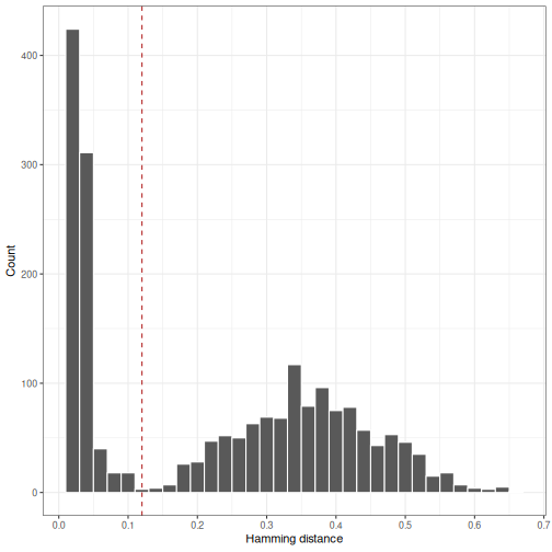
By manual inspection, the length normalized ham model distance threshold would be
set to a value near 0.12 in the above example.
# Generate HH_S5F distance histogram
p2 <- ggplot(subset(dist_s5f, !is.na(dist_nearest)),
             aes(x=dist_nearest)) +
    theme_bw() +
    xlab("HH_S5F distance") +
    ylab("Count") +
    scale_x_continuous(breaks=seq(0, 50, 5)) +
    geom_histogram(color="white", binwidth=1) +
    geom_vline(xintercept=7, color="firebrick", linetype=2)
plot(p2)
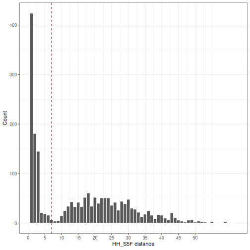
In this example, the unnormalized hh_s5f model distance threshold would be
set to a value near 7.
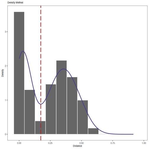
Automated threshold detection via smoothed density
The density method will look for the minimum in the valley between two modes of a smoothed
distribution based on the input vector (distances), which will generally be the
dist_nearest column from the distToNearest output. Below is an example of using the
density method for threshold detection.
# Find threshold using density method
output <- findThreshold(dist_ham$dist_nearest, method="density")
threshold <- output@threshold

# Plot distance histogram, density estimate and optimum threshold
plot(output, title="Density Method")
# Print threshold
print(output)
## [1] 0.1738391
Automated threshold detection via a mixture model
The findThreshold function includes approaches for automatically determining
a clonal assignment threshold. The "gmm" method (gamma/Gaussian mixture method)
of findThreshold (method="gmm") performs a maximum-likelihood fitting
procedure over the distance-to-nearest distribution using one of four combinations of
univariate density distribution functions: "norm-norm" (two Gaussian distributions),
"norm-gamma" (lower Gaussian and upper gamma distribution),
"gamma-norm" (lower gamm and upper Gaussian distribution), and "gamma-gamma"
(two gamma distributions). By default, the threshold will be selected by calculating
the distance at which the average of sensitivity and specificity reaches its maximum
(cutoff="optimal"). Alternative threshold selection criteria are also providing, including
the curve intersection (cutoff="intersect"), user defined sensitivity
(cutoff="user", sen=x), or user defined specificity (cutoff="user", spc=x)
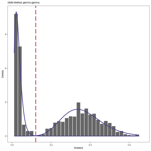
In the example below the mixture model method (method="gmm") is used to find the optimal
threshold for separating clonally related sequences by fitting two gamma distributions
(model="gamma-gamma"). The red dashed-line shown in figure below defines the distance
where the average of the sensitivity and specificity reaches its maximum.
# Find threshold using gmm method
output <- findThreshold(dist_ham$dist_nearest, method="gmm", model="gamma-gamma")

# Plot distance histogram, Gaussian fits, and optimum threshold
plot(output, binwidth=0.02, title="GMM Method: gamma-gamma")
# Print threshold
print(output)
## [1] 0.1214102
Note: The shape of histogram plotted by plotGmmThreshold is governed
by the binwidth parameter. Meaning, any change in bin size will change the
form of the distribution, while the gmm method is
completely bin size independent and only engages the real input data.
Calculating nearest neighbor distances independently for subsets of data
The fields argument to distToNearest will split the input data.frame
into groups based on values in the specified fields (columns) and will
treat them independently. For example, if the input data has multiple
samples, then fields="sample_id" would allow each sample to be analyzed
separately.
In the previous examples we used a subset of the original example data. In the
following example, we will use the two available samples, -1h and +7d,
and will set fields="sample_id". This will reproduce previous results for sample
-1h and add results for sample +7d.
dist_fields <- distToNearest(ExampleDb, model="ham", normalize="len",
                             fields="sample_id", nproc=1)
We can plot the nearest neighbor distances for the two samples:
# Generate grouped histograms
p4 <- ggplot(subset(dist_fields, !is.na(dist_nearest)),
             aes(x=dist_nearest)) +
    theme_bw() +
    xlab("Grouped Hamming distance") +
    ylab("Count") +
    geom_histogram(color="white", binwidth=0.02) +
    geom_vline(xintercept=0.12, color="firebrick", linetype=2) +
    facet_grid(sample_id ~ ., scales="free_y")
plot(p4)
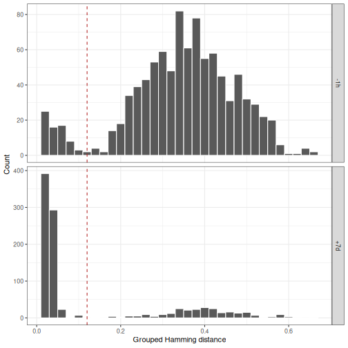
In this case, the threshold selected for -1h seems to work well
for +7d as well.
Calculating nearest neighbor distances across groups rather than within a groups
Specifying the cross argument to distToNearest forces distance calculations
to be performed across groups, such that the nearest neighbor of each sequence
will always be a sequence in a different group. In the following example
we set cross="sample", which will group the data into -1h and
+7d sample subsets. Thus, nearest neighbor distances for sequences in sample
-1h will be restricted to the closest sequence in sample +7d and vice versa.
dist_cross <- distToNearest(ExampleDb, sequenceColumn="junction",
                            vCallColumn="v_call_genotyped", jCallColumn="j_call",
                            model="ham", first=FALSE,
                            normalize="len", cross="sample_id", nproc=1)
# Generate cross sample histograms
p5 <- ggplot(subset(dist_cross, !is.na(cross_dist_nearest)),
             aes(x=cross_dist_nearest)) +
    theme_bw() +
    xlab("Cross-sample Hamming distance") +
    ylab("Count") +
    geom_histogram(color="white", binwidth=0.02) +
    geom_vline(xintercept=0.12, color="firebrick", linetype=2) +
    facet_grid(sample_id ~ ., scales="free_y")
plot(p5)
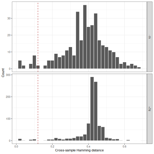
This can provide a sense of overlap between samples or a way to compare within-sample variation to cross-sample variation.
Speeding up pairwise-distance-matrix calculations with subsampling
The subsample option in distToNearest allows to speed up calculations and
reduce memory usage.
If there are very large groups of sequences that share V call, J call and junction length,
distToNearest will need a lot of memory and it will take a long time to calculate all
the distances. Without subsampling, in a large group of n=70,000 sequences
distToNearest calculates a n*n distance matrix. With subsampling, e.g. to s=15,000,
the distance matrix for the same group has size s*n, and for each sequence in db,
the distance value is calculated by comparing the sequence to the subsampled sequences
from the same V-J-junction length group.
# Explore V-J-junction length groups sizes to use subsample
# Show the size of the largest groups
library(dplyr)
##
## Attaching package: 'dplyr'
## The following objects are masked from 'package:stats':
##
##     filter, lag
## The following objects are masked from 'package:base':
##
##     intersect, setdiff, setequal, union
library(alakazam)
top_10_sizes <- ExampleDb %>%
     group_by(junction_length) %>% # Group by junction length
     do(alakazam::groupGenes(., first=TRUE)) %>% # Group by V and J call
     mutate(GROUP_ID=paste(junction_length, vj_group, sep="_")) %>% # Create group ids
     ungroup() %>%
     group_by(GROUP_ID) %>% # Group by GROUP_ID
     distinct(junction) %>% # Count unique junctions per group
     summarize(SIZE=n()) %>% # Get the size of the group
     arrange(desc(SIZE)) %>% # Sort by decreasing size
     select(SIZE) %>%
     top_n(10) # Filter to the top 10
## Selecting by SIZE
top_10_sizes
## # A tibble: 10 × 1
##     SIZE
##    <int>
##  1    89
##  2    37
##  3    36
##  4    34
##  5    33
##  6    33
##  7    32
##  8    26
##  9    25
## 10    25
# Use 30 to subsample
# NOTE: This is a toy example. Subsampling to 30 sequence with real data is unwise
dist <- distToNearest(ExampleDb, sequenceColumn="junction",
                      vCallColumn="v_call_genotyped", jCallColumn="j_call",
                      model="ham",
                      first=FALSE, normalize="len",
                      subsample=30)