Selection quantification
BASELINe quantifies selection pressure by calculating the posterior probability density function (PDF) based on observed mutations compared to expected mutation rates derived from an underlying SHM targeting model. Selection is quantified via the following steps:
- Calculate the selection scores for individual sequences.
- Group by relevant fields for comparison and convolve individual selection PDFs.
- Plot and compare selection scores of different groups of sequences.
Example data
A small example AIRR Rearrangement database is included in the alakazam package.
The example dataset consists of a subset of Ig sequencing data from an
influenza vaccination study (Laserson and Vigneault et al., PNAS, 2014). The
data include sequences from multiple time-points before and after the subject
received an influenza vaccination. Quantifying selection requires the following
fields (columns) to be present in the table:
sequence_idsequence_alignmentgermline_alignment_d_mask
# Import required packages
library(alakazam)
library(shazam)

# Load and subset example data (for faster demonstration)
data(ExampleDb, package="alakazam")
ExampleDb <- subset(ExampleDb, c_call %in% c("IGHA", "IGHG"))
Preprocessing
Before starting the selection analysis, data need to be prepared in one of two ways:
-
Constructing clonal consensus sequences.
-
Incorporating lineage information.
Constructing clonal consensus sequences
Individual sequences within clonal groups are not, strictly speaking,
independent events and it is generally appropriate to only analyze selection
pressures on an effective sequence for each clonal group. The collapseClones
function provides one strategy for generating an effective sequences for
each clone. It reduces the input database to one row per clone and appends
clonal_sequence and clonal_germline columns which contain the
consensus sequences for each clone.
# Collapse clonal groups into single sequences
clones <- collapseClones(ExampleDb, cloneColumn="clone_id",
                         sequenceColumn="sequence_alignment",
                         germlineColumn="germline_alignment_d_mask",
                         regionDefinition=IMGT_V,
                         method="thresholdedFreq", minimumFrequency=0.6,
                         includeAmbiguous=FALSE, breakTiesStochastic=FALSE,
                         nproc=1)
Incorporating lineage information
For each clone, lineage information can be incorporated following these steps:
# Subset to sequences with clone_id=3170
db_3170 <- subset(ExampleDb, clone_id == 3170)
dim(db_3170)
colnames(db_3170)

# Generate a ChangeoClone object for lineage construction
clone_3170 <- makeChangeoClone(db_3170, seq="sequence_alignment", germ="germline_alignment")

# Run the lineage reconstruction
dnapars_exec <- "/usr/local/bin/dnapars"
graph_3170 <- buildPhylipLineage(clone_3170, dnapars_exec, rm_temp=TRUE)

# Generating a data.frame from the lineage tree graph object,
# and merge it with clone data.frame
graph_3170_df <- makeGraphDf(graph_3170, clone_3170)
dim(graph_3170_df)
colnames(graph_3170_df)
makeGraphDf creates a data.frame with the column parent_sequence, which can be used to analyze
mutations for each sequence relative to their parent_sequence.
Calculate selection PDFs for individual sequences
Selection scores are calculated with the calcBaseline function. This can
be performed with a single call to calcBaseline, which performs all
required steps. Alternatively, one can perform each step separately for
greater control over the analysis parameters.
Calculating selection in multiple steps
Following construction of an effective sequence for each clone, the observed
and expected mutation counts are calculated for each sequence in the
clonal_sequence column relative to the clonal_germline. observedMutations
is used to calculate the number of observed mutations and
expectedMutations calculates the expected frequency of mutations.
The underlying targeting model for calculating expectations can be specified
using the targetingModel parameter. In the example below, the default
HH_S5F is used. Column names for sequence and germline sequence may
also be passed in as parameters if they differ from the Change-O defaults.
Mutations are counted by these functions separately for complementarity
determining (CDR) and framework (FWR) regions. The regionDefinition
argument defines whether these regions are handled separately, and where
the boundaries lie. There are several built-in region definitions
in the shazam package, both dependent upon the V segment
being IMGT-gapped:
IMGT_V: All regions in the V segment, excluding CDR3, grouped as either CDR or FWR.IMGT_V_BY_REGIONS: The CDR1, CDR2, FWR1, FWR and FWR3 regions in the V segment (no CDR3) treated as individual regions.IMGT_VDJ: All regions, including CDR3 and FWR4, grouped as either CDR or FWR. ThisRegionDefinitionis initially empty, and one is created on the fly for each set of clonally related sequences.IMGT_VDJ_BY_REGIONS: CDR1, CDR2, CDR3, FWR1, FWR, FWR3 and FWR4 regions treated as individual regions. ThisRegionDefinitionis initially empty, and one is created on the fly for each set of clonally related sequences.
Users may define other region sets and boundaries by creating a custom
RegionDefinition object.
# Count observed mutations and append mu_count columns to the output
observed <- observedMutations(clones,
                              sequenceColumn="clonal_sequence",
                              germlineColumn="clonal_germline",
                              regionDefinition=IMGT_V, nproc=1)
# Count expected mutations and append mu_exptected columns to the output
expected <- expectedMutations(observed,
                              sequenceColumn="clonal_sequence",
                              germlineColumn="clonal_germline",
                              targetingModel=HH_S5F,
                              regionDefinition=IMGT_V, nproc=1)
The counts of observed and expected mutations can be combined to test for selection
using calcBaseline. The statistical framework used to test for selection based
on mutation counts can be specified using the testStatistic parameter.
# Calculate selection scores using the output from expectedMutations
baseline <- calcBaseline(expected, testStatistic="focused",
                         regionDefinition=IMGT_V, nproc=1)
## calcBaseline will use existing observed and expected mutations, in the fields: mu_count_cdr_r, mu_count_cdr_s, mu_count_fwr_r, mu_count_fwr_s and mu_expected_cdr_r, mu_expected_cdr_s, mu_expected_fwr_r, mu_expected_fwr_s
Calculating selection in one step
It is not required for observedMutation and expectedMutations to be run prior to
calcBaseline. If the output of these two steps does not appear in the input
data.frame, then calcBaseline will call the appropriate functions prior to
calculating selection scores.
# Calculate selection scores from scratch
baseline <- calcBaseline(clones, testStatistic="focused",
                         regionDefinition=IMGT_V, nproc=1)
Using alternative mutation definitions and models
The default behavior of observedMutations and expectedMutations, and
by extension calcBaseline, is to define a replacement mutation in the usual
way - any change in the amino acid of a codon is considered a replacement
mutation. However, these functions have a mutationDefinition argument which
allows these definitions to be changed by providing a MutationDefinition
object that contains alternative replacement and silent criteria. shazam
provides the following built-in MutationDefinition objects:
CHARGE_MUTATIONS: Amino acid mutations are defined by changes in side chain charge class.HYDROPATHY_MUTATIONS: Amino acid mutations are defined by changes in side chain hydrophobicity class.POLARITY_MUTATIONS: Amino acid mutations are defined by changes in side chain polarity class.VOLUME_MUTATIONS: Amino acid mutations are defined by changes in side chain volume class.
The default behavior of expectedMutations is to use the human 5-mer mutation model,
HH_S5F. Alternative SHM targeting models can be provided using the
targetingModel argument.
# Calculate selection on charge class with the mouse 5-mer model
baseline_mk_rs5nf <- calcBaseline(clones, testStatistic="focused",
                         regionDefinition=IMGT_V,
                         targetingModel=MK_RS5NF,
                         mutationDefinition=CHARGE_MUTATIONS,
                         nproc=1)
Group and convolve individual selection distributions
To compare the selection scores of groups of sequences, the sequences must
be convolved into a single PDF representing each group. In the example dataset,
the sample_id field corresponds to samples taken at different time points
before and after an influenza vaccination and the c_call field specifies
the isotype of the sequence. The groupBaseline function convolves the BASELINe
PDFs of individual sequences/clones to get a combined PDF. The field(s) by
which to group the sequences are specified with the groupBy parameter.
The groupBaseline function automatically calls summarizeBaseline to
generate summary statistics based on the requested groupings, and populates
the stats slot of the input Baseline object with the number of sequences
with observed mutations for each region, mean selection scores, 95% confidence
intervals, and p-values with positive signs indicating the presence of positive
selection and/or p-values with negative signs indicating the presence of negative
selection. The magnitudes of the p-values (without the signs) should be
interpreted as analogous to a t-test.
Grouping by a single annotation
The following example generates a single selection PDF for each unique
annotation in the sample_id column.
# Combine selection scores by time-point
grouped_1 <- groupBaseline(baseline, groupBy="sample_id")
Subsetting and grouping by multiple annotations
Grouping by multiple annotations follows the sample procedure as a
single annotation by simply adding columns to the groupBy argument.
Subsetting the data can be performed before or after generating selection
PDFs via calcBaseline. However, note that subsetting may impact the clonal
representative sequences generated by collapseClones. In the following
example, subsetting precedes the collapsing of clonal groups.
# Subset the original data to switched isotypes
db_sub <- subset(ExampleDb, c_call %in% c("IGHM", "IGHG"))

# Collapse clonal groups into single sequence
clones_sub <- collapseClones(db_sub, cloneColumn="clone_id",
                             sequenceColumn="sequence_alignment",
                             germlineColumn="germline_alignment_d_mask",
                             regionDefinition=IMGT_V,
                             method="thresholdedFreq", minimumFrequency=0.6,
                             includeAmbiguous=FALSE, breakTiesStochastic=FALSE,
                             nproc=1)

# Calculate selection scores from scratch
baseline_sub <- calcBaseline(clones_sub, testStatistic="focused",
                             regionDefinition=IMGT_V, nproc=1)
## calcBaseline will calculate observed and expected mutations for clonal_sequence using clonal_germline as a reference.
# Combine selection scores by time-point and isotype
grouped_2 <- groupBaseline(baseline_sub, groupBy=c("sample_id", "c_call"))
Convolving variables at multiple levels
To make selection comparisons using two levels of variables, you
would need two iterations of groupings, where the first iteration of
groupBaseline groups on both variables, and the second iteration groups
on the “outer” variable. For example, if a data set has both case and control
subjects annotated in status and subject columns, then
generating convolved PDFs for each status would be performed as:
# First group by subject and status
subject_grouped <- groupBaseline(baseline, groupBy=c("status", "subject"))

# Then group the output by status
status_grouped <- groupBaseline(subject_grouped, groupBy="status")
Testing the difference in selection PDFs between groups
The testBaseline function will perform significance testing between two
grouped BASELINe PDFs, by region, and return a data.frame with the
following information:
region: The sequence region, such ascdrandfwr.test: The name of the two groups compared.pvalue: Two-sided p-value for the comparison.fdr: FDR corrected p-value.
testBaseline(grouped_1, groupBy="sample_id")
##   region       test     pvalue        fdr
## 1    cdr -1h != +7d 0.04494357 0.08988715
## 2    fwr -1h != +7d 0.49922881 0.49922881
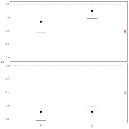
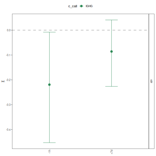
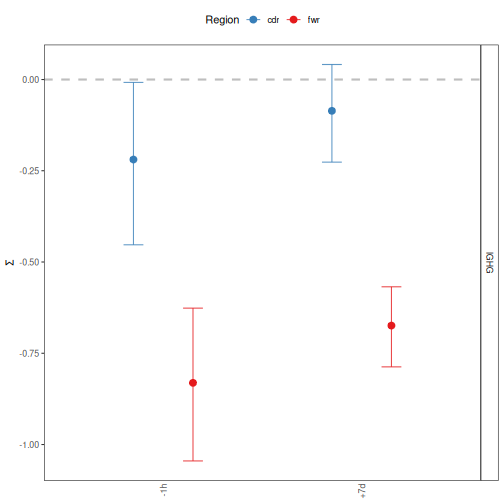
Plot and compare selection scores for groups
plotBaselineSummary plots the mean and confidence interval of selection scores
for the given groups. The idColumn argument specifies the field that contains
identifiers of the groups of sequences. If there is a secondary field by which
the sequences are grouped, this can be specified using the groupColumn. This
secondary grouping can have a user-defined color palette passed into
groupColors or can be separated into facets by setting the facetBy="group".
The subsetRegions argument can be used to visualize selection of specific
regions. Several examples utilizing these different parameters are provided
below.
# Set sample and isotype colors
sample_colors <- c("-1h"="seagreen", "+7d"="steelblue")
isotype_colors <- c("IGHM"="darkorchid", "IGHD"="firebrick",
                    "IGHG"="seagreen", "IGHA"="steelblue")

# Plot mean and confidence interval by time-point
plotBaselineSummary(grouped_1, "sample_id")
# Plot selection scores by time-point and isotype for only CDR
plotBaselineSummary(grouped_2, "sample_id", "c_call", groupColors=isotype_colors,
                    subsetRegions="cdr")
# Group by CDR/FWR and facet by isotype
plotBaselineSummary(grouped_2, "sample_id", "c_call", facetBy="group")
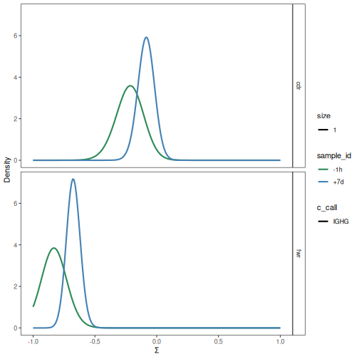
plotBaselineDensity plots the full Baseline PDF of selection scores for the
given groups. The parameters are the same as those for plotBaselineSummary.
However, rather than plotting the mean and confidence interval, the full density
function is shown.
# Plot selection PDFs for a subset of the data
plotBaselineDensity(grouped_2, "c_call", groupColumn="sample_id", colorElement="group",
                    colorValues=sample_colors, sigmaLimits=c(-1, 1))
Editing a field in a Baseline object
If for any reason you need to edit the existing values in a field in a
Baseline object, you can do so via editBaseline. In the following example,
we remove results related to IGHA in the relevant fields from grouped_2.
When the input data is large and it takes a long time for calcBaseline to run,
editBaseline could become useful when, for instance, you would like to exclude
a certain sample or isotype, but would rather not re-run calcBaseline after
removing that sample or isotype from the original input data.
# Get indices of rows corresponding to IGHA in the field "db"
# These are the same indices also in the matrices in the fileds "numbOfSeqs",
# "binomK", "binomN", "binomP", and "pdfs"
# In this example, there is one row of IGHA for each sample
dbIgMIndex <- which(grouped_2@db[["c_call"]] == "IGHG")

grouped_2 <- editBaseline(grouped_2, "db", grouped_2@db[-dbIgMIndex, ])
grouped_2 <- editBaseline(grouped_2, "numbOfSeqs", grouped_2@numbOfSeqs[-dbIgMIndex, ])
grouped_2 <- editBaseline(grouped_2, "binomK", grouped_2@binomK[-dbIgMIndex, ])
grouped_2 <- editBaseline(grouped_2, "binomN", grouped_2@binomN[-dbIgMIndex, ])
grouped_2 <- editBaseline(grouped_2, "binomP", grouped_2@binomP[-dbIgMIndex, ])
grouped_2 <- editBaseline(grouped_2, "pdfs",
                          lapply(grouped_2@pdfs, function(pdfs) {pdfs[-dbIgMIndex, ]} ))

# The indices corresponding to IGHA are slightly different in the field "stats"
# In this example, there is one row of IGHA for each sample and for each region
grouped_2 <- editBaseline(grouped_2, "stats",
                          grouped_2@stats[grouped_2@stats[["c_call"]] != "IGHA", ])